Concepts

The base model in ClimateRisk is CLIMADA, in this section, we provide a brief about several concepts about CLIMADA. Detailsa about how to use CLIMADA can be obtained from CLIMADA documentation.

1. Exposure

1.1 Input data

Exposure describes the set of assets, people, livelihoods, infrastructures, etc. within an area of interest in terms of their geographic location, their value etc.; in brief - everything potentially exposed to hazards. In ClimateRisk, Exposure must be read as a shp file (it contains objects such as LineString or Point).

For example, in etc/data there are three types of Exposures:

• lds-nz-railway-centre-lines-SHP: New Zealand railway lines.

• lds-nz-road-centrelines-topo-150k-SHP: New Zealand all roads (centre lines).

• nz-state-highway-centrelines-2012-SHP: New Zealand state highways (centre lines).

We can choose the shp file in the configuration file, for example,

...

input:
    file: etc/data/nz-state-highway-centrelines-2012-SHP/nz-state-highway-centrelines-2012.shp
    ...
...

1.2 Exposure value

By default, the value of the above Exposures (for each segment) is 1.0. However it can be overwriten using references from

• LitPop: it is used to initiate grided exposure data (with estimates of either asset value, economic activity or population) based on nightlight intensity (Lit) and population count (Pop) data. Details can be obtained here.

• GDP: the exposed assets are calculated by means of national GDP converted to total national wealth as a proxy for asset distribution.

• fixed value: a user defined fixed value can be applied to Exposures.

The Exposures value can be configued in the value_adjustment_option section, for example,

...

input:
    ...
    value_adjustment_option:
        litpop: null
        gdp2asset: null
        fix:
            method: individual  # it can be set to individual or total
            value: 30

litpop, gdp2asset and value cannot be set to True at the same time. In the fix section, we need to set whether we want to apply value (in the above configuration it is 30) over the entire Exposures (method: total), or for each segment (method: individual).

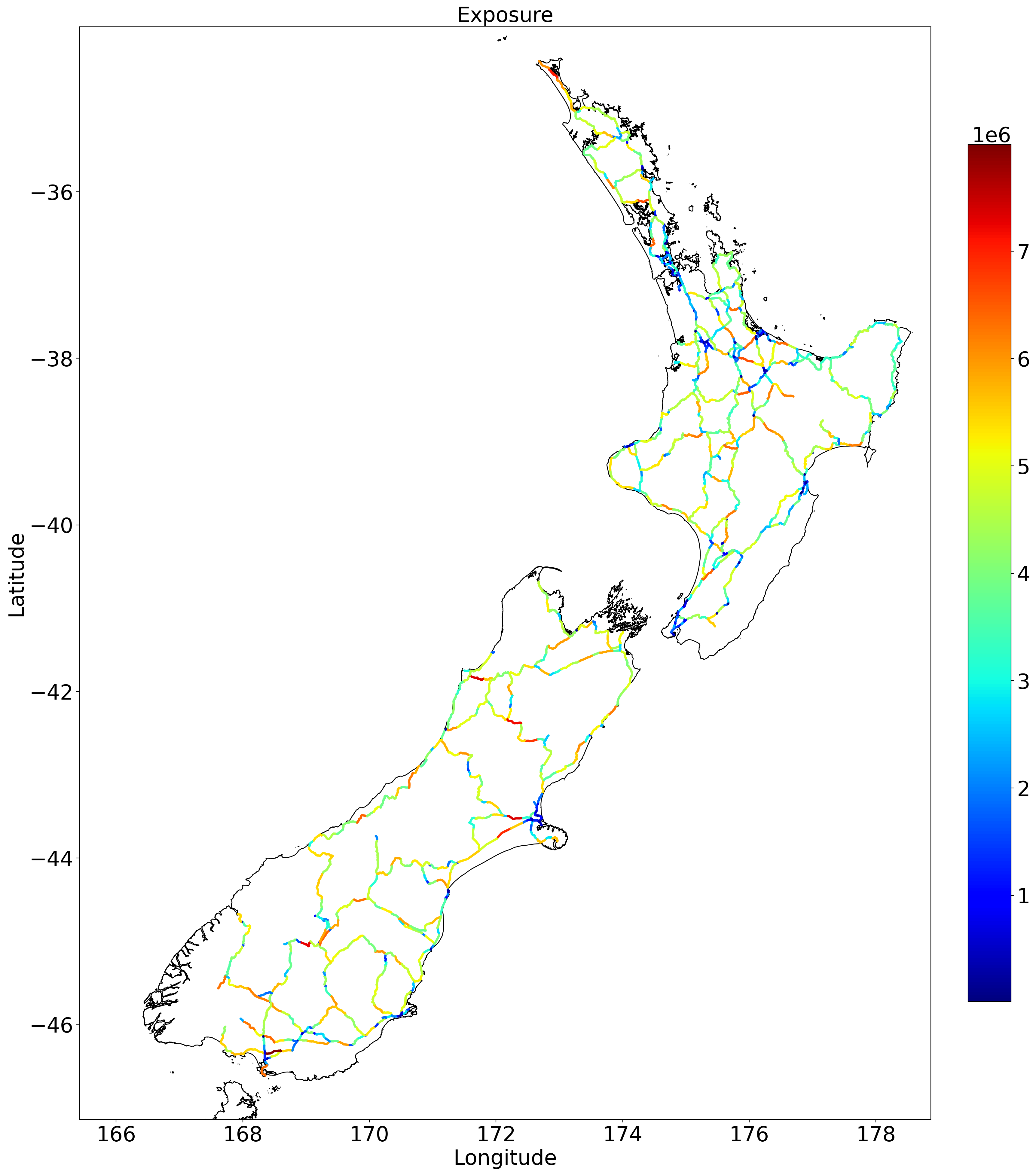
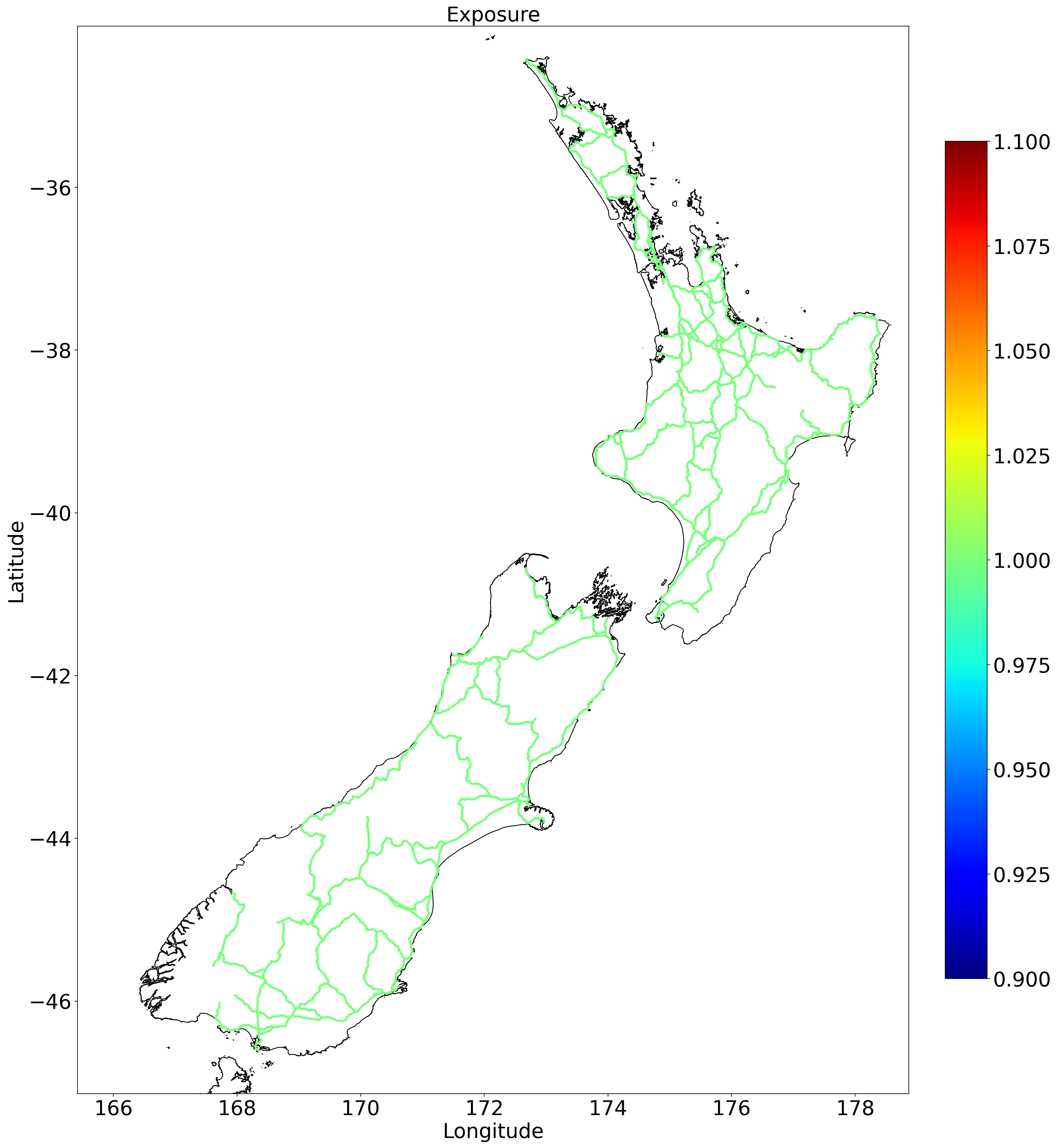
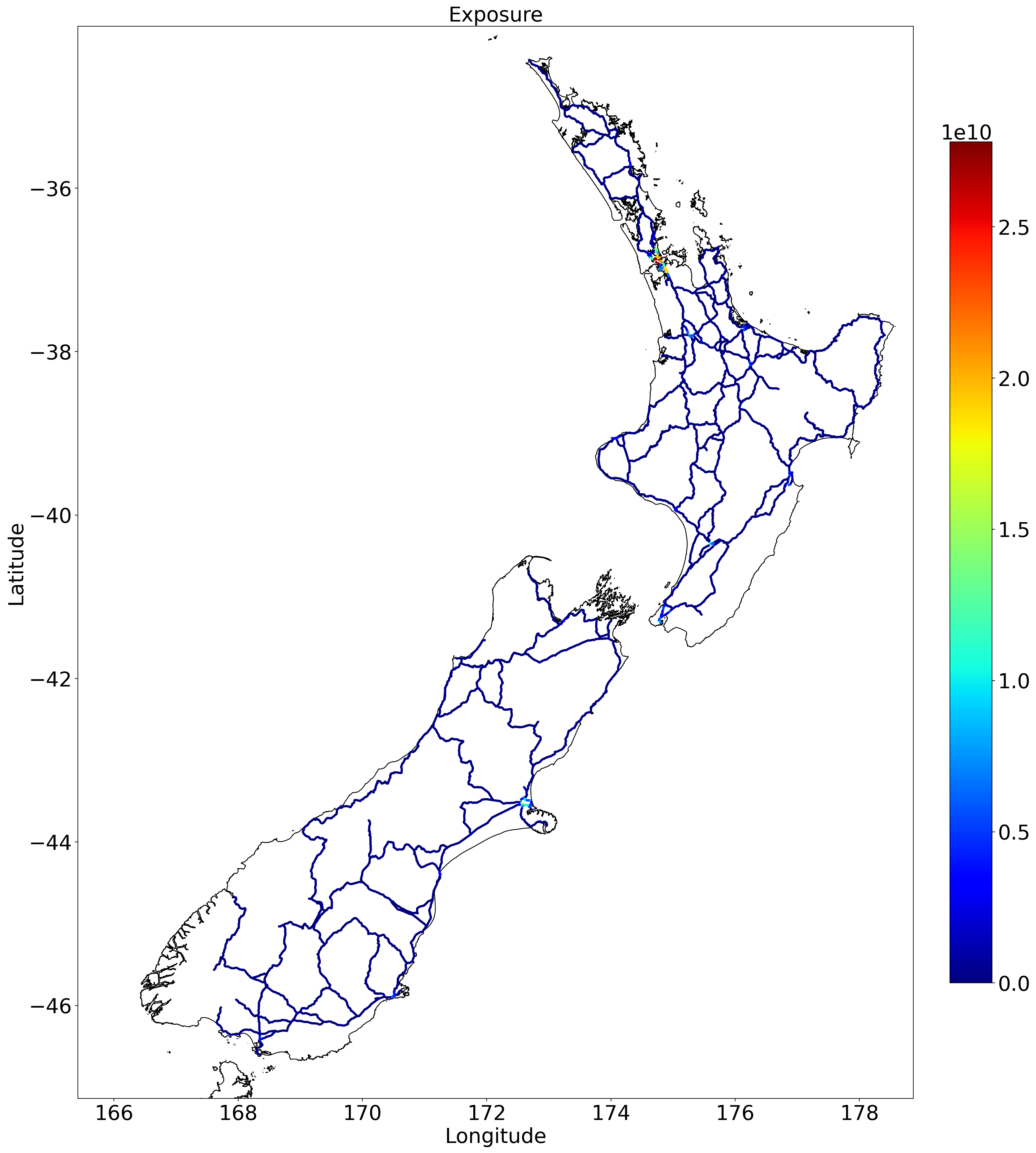
Examples for the New Zealand State Highway with different exposure setups are shown below:

• left: with a total state highway asset value of $52b.

• middle: with a fixed segment value of $1.0.

• right: using Litpop to represent the value.

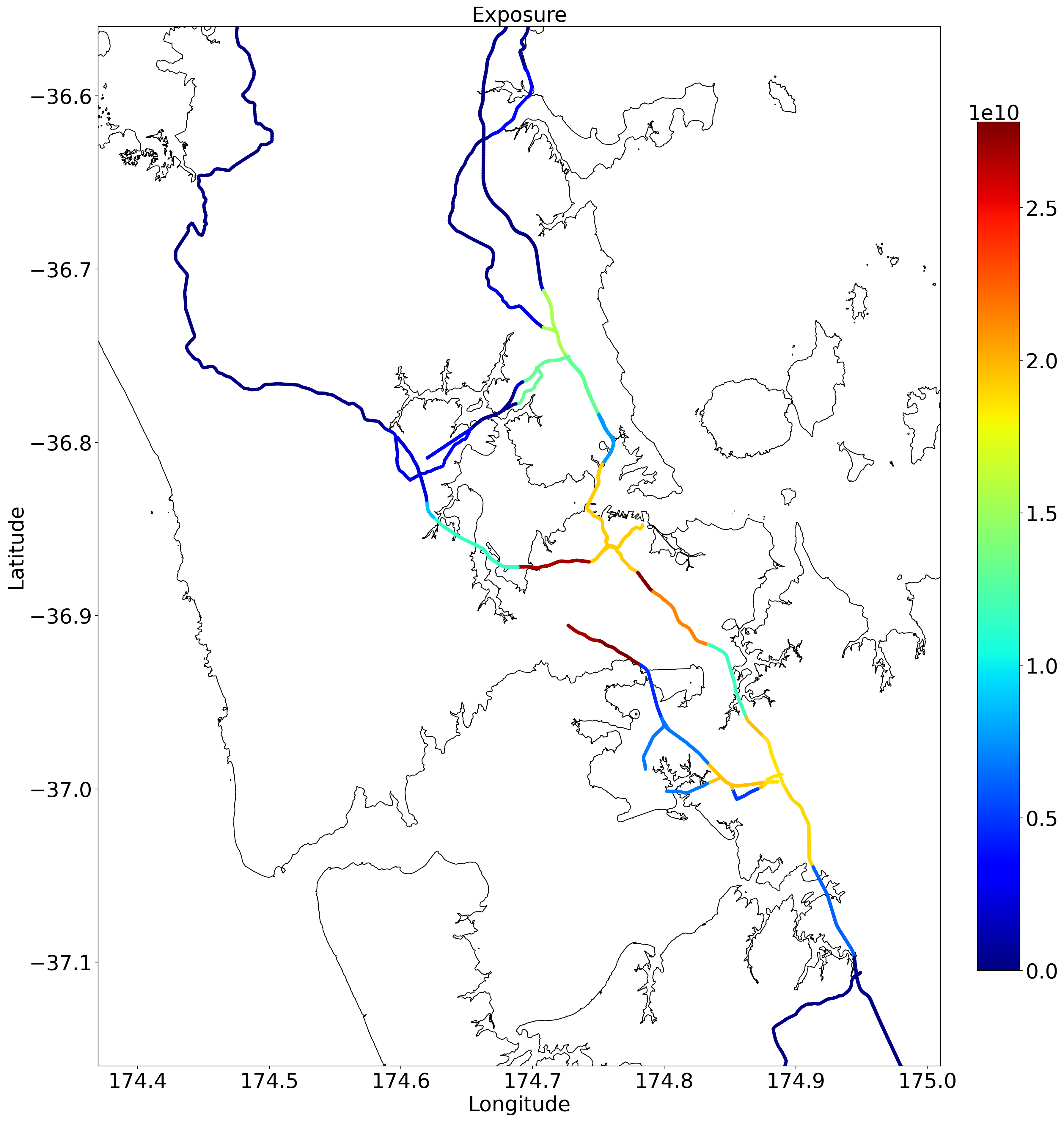
The following figure shows the zoomed-in state highway in Auckland (with litpop):

2. Hazard

Hazard defines the climate hazards that are used to assess the impacts on the Exposure. Currently in ClimateRisk, three types of hazards are pre-defined: TC, Flood and Landslide.

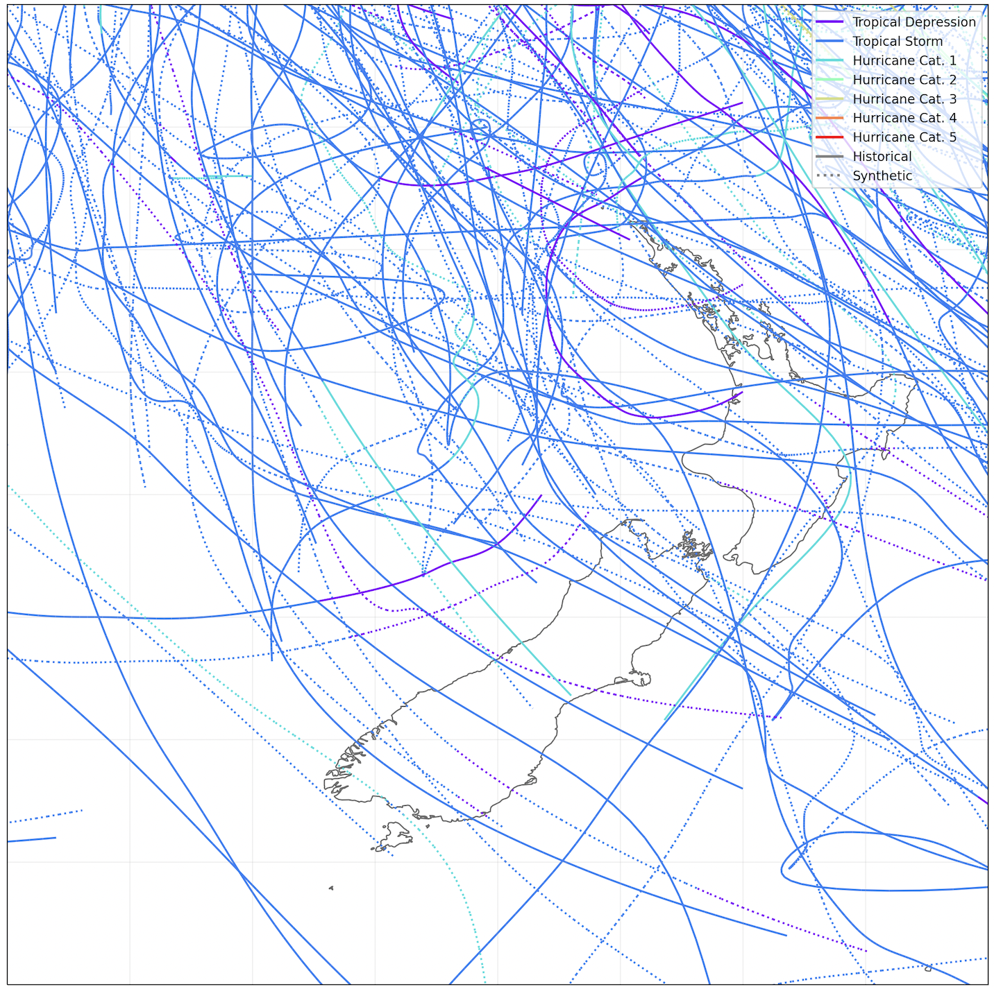
2.1 Tropical cyclone (TC)

A total of 175 years (up to 2022) Tropical cyclone (TC) records are used. Additionally, pertubated cyclone tracks are added in the dataset. Note that the dataset might not be comprehensive. An example of TC tracks is shown below:

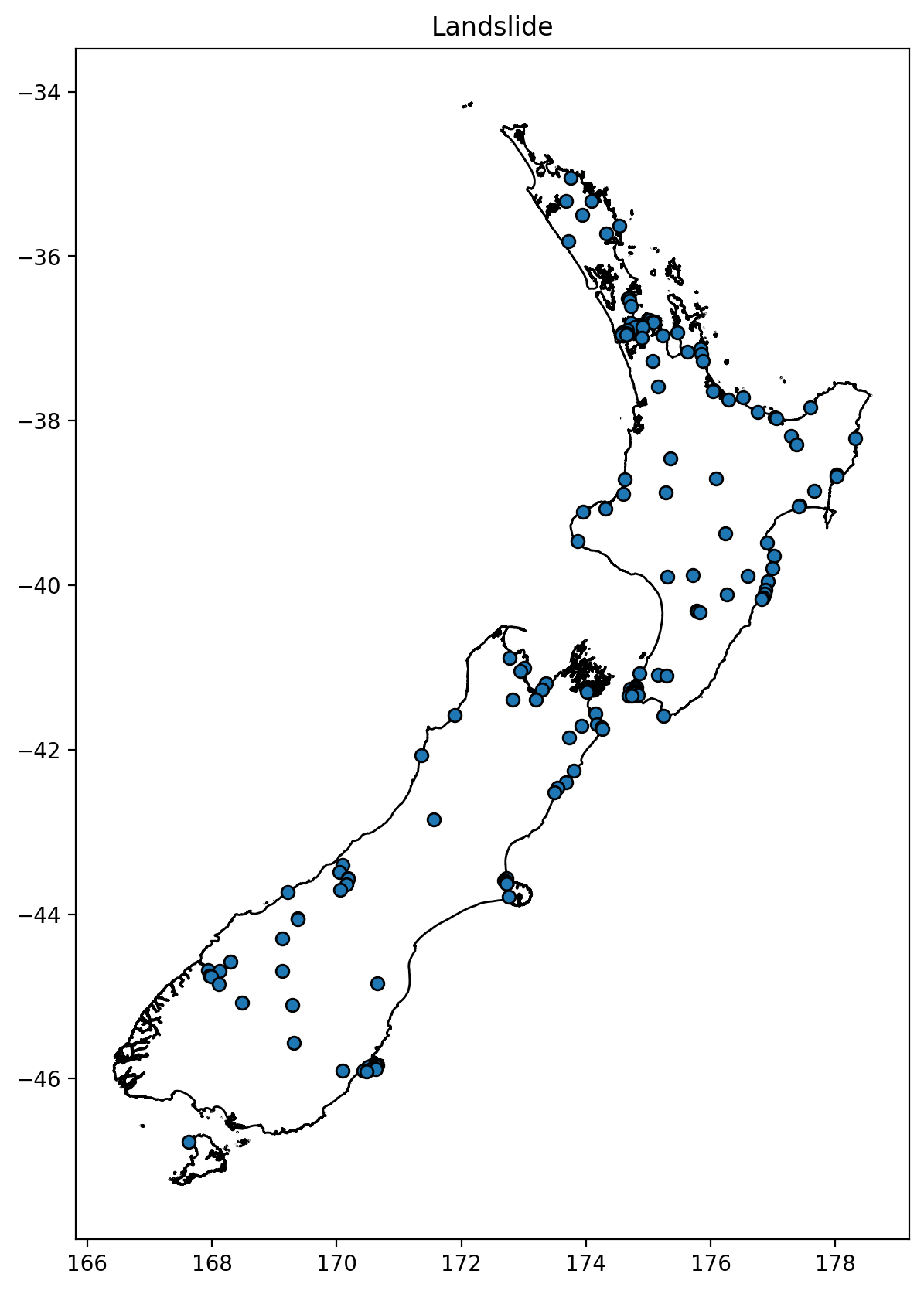
2.2 Landslide

Landslide is obtained from NASA Global Landslide Catalog (Points). It records most landslides globally. For New Zealand, there are a total of 164 events recorded spanning from 1979 to 2018. All the events are shown below:

2.3 Flood

The runoff was used to derive spatially explicit flood depth (FLDDPH) and flooded fraction (FLDFRC) of the maximum flood event of each year on 150 arcsec (~ 5 km). For the New Zealand events, a total of 40 events spanning from 1971 and 2010 are recorded.

The type of Hazard can be defined in the configuration file. For example, in the following configuration file landslide is enabled in ClimateRisk:

...

hazard:
    flood:
        enable: False
    landslide:
        enable: True
    TC_track:
        enable: False
...

Note that there is an API provided by CLIMADA to easily extract hazard data (for types such as tropical_cyclone, earthquake, river_flood, wildfire, flood). Details can be obtained at Climada-petals.

3. Impact function

An impact function relates the percentage of damage in the exposure caused by an hazard (or a type of hazard). It is also referred as a “vulnerability curve” in the modelling community.

There are two main metrics in a impact function:

• MDD: Mean damage (impact) degree for each intensity.

• PAA: Percentage of affected assets (exposures) for each intensity.

• MDR: MDR=MDD * PAA is the mean damage ratio.

There are a few predefined impact functions in ClimateRisk (by CLIMADA).

3.1 Tropical cyclone (TC)

For Tropical cyclone, the impact function is defined using Emanuel (2011).

The above figure shows that the analysis TC intensity range (wind speed) is between 0 m/s and 120 m/s. PAA is always 100%, meaning that all areas of exposure will be affected if there is a TC event. MDD indicates that the TC start brining more significant impact when the TC intensity is more than 40 m/s.

3.2 Landslide

For landslide, an customized impact function is defined (in process/impact.py).

The intensity of landside is ranging from 0 to 1. When a landslide occurs, all areas of exposure will be affected while it only brings significant impacts when the landslide intensity is more than 0.5.

3.3 Flood

For flood, the following impact function is defined as below

The unit of flood intensity is m, when the intensity is over approximate 1 m, the impact (e.g., MDD) from the event signifciantly increases.

In ClimateRisk, impact function is automatically determined by the predefined hazard type.

4. Cost benefit

Cost benefit allows an user to compare different hazard adaptation options.

• When a cost-benefit ratio < 1, the cost is less than the benefit so the adaptation approach is considered a worthwhile investment (Smaller ratios therefore represent better investments).

• When a cost-benefit ratio > 1, the cost is more than the benefit and the offset losses are less than the cost of the adaptation measure: based on the financials alone (the measure may not be worth it).

4.1 A simple cost-benefit

\[\frac{cost}{benefit} = \frac{cost}{N * (AAI^{without adaptation} - AAI^{with adaptation})}\]

Where N is the number of years, the AAI is the Average Annual Impact from your hazard event set on the exposure.

Note

Whether an adaptation measure is seen to be effective might depend on the number of years you are evaluating the cost-benefit over. For example, a $50 investment that prevents an average of $1 losses per year will only “break even” after N=50 years. Details can be accessed from CLIMADA.

4.2 Time dependant cost-benefit

Sometimes Cost-benefit calculation will want to describe a climate and exposure that also change over time. In such case, it does not assume that the user will have explicit hazard and impact objects for every year in the study period, and so interpolates between the impacts at the start and the end of the period of interest.

\[\sum_{t=T_0}^{T_1} a(t)(AAI^{with adaptation}_{T_1} - AAI^{with adaptation}_{T_0} ) - N * AAI^{without adaptation}_{T_0}\]

Where a(t) is a function of the year t describing the interpolation of hazard and exposure between \(T_0\) and \(T_1\). It is usually defined as:

\[a_{k}(t) = \frac{(t - T_0)^{k}} {T_1 - T_0}^{k}\]

the choice (usually defined by user) determins how quickly the transition occurs between the present and future:

• k=1: the function is a straightline (the change rate over time is stable).

• k>1: the change begins slowly and speeds up over time.

• k<1: the change begins quickly and slows over time.

4.3 Discount rates

The discount rate tries to formalise an idea from economics that says that a gain in the future is worth less to us than the same gain right now. For example, paying $1 to offset $2 of economic losses next year is worth more than paying $1 to offset $2 of economic losses in 2080.

There are three main ideas around discount rates:

• The most widley used discount rate in climate change economics is 1.4% as proposed by the Stern Review (2006).

• Neoliberal economists around Nordhaus (2007) claim that rates should be higher, around 4.3%, reflecting continued economic growth and a society that will be better at adapting in the future compared to now.

• Environmental economists argue that future costs shouldn not be discounted at all.

The discount rates can be considered in Cost-benefits calculation, details can be accessed here.

5. Adaptation

Adaptation measures are defined by parameters that alter the exposures, hazard or impact functions.

An adapation measure is usually described as:

• Description:

  • name: name of the action.

  • haz_type: hazard type (e.g., landslide).

  • cost: discounted cost repqted to the exposure.

• Source:

  • hazard_set: file name of hazard to use (in h5 format).

  • exposure_set: file name of exposure to use (in h5 format).

• impact functions transformation:

  • hazard_inten_imp: parameter a and b of hazard intensity change (in tuple).

  • mdd_impact: parameter a and b of the impact over the mean damage degree (in tuple).

  • paa_impact: parameter a and b of the impact over the percentage of affected assets (in tuple).

All three aspects in a impact function can be modified using the above three parameters:

intensity = intensity*hazard_inten_imp[0] + hazard_inten_imp[1]
mdd = mdd*mdd_impact[0] + mdd_impact[1]
paa = paa*paa_impact[0] + paa_impact[1]

• Hazard modification:

• hazard_freq_cutoff: hazard frequency cutoff (in float): the hazard intensity is set to 0 when its impact exceedance frequency are greater than hazard_freq_cutoff.

• imp_fun_map: change of impact function id.

• exp_region_id: region id of the selected exposures to consider ALL the previous parameters.

• risk_transf_attach: risk transfer attachment. Applies to the whole exposure.

• risk_transf_cover: risk transfer cover. Applies to the whole exposure.

The adapation is configurated via the adaptation configuration section. For example,

adaptation:
    TC_wind:
        measure1:
            mdd_impact: (1, 0)
            paa_impact: (1, -0.15)
            hazard_inten_imp: (1, -10)
            cost: 10000
            color_rgb: (1, 1, 1)
            discount_rate: 0.014

Here the adapation measure for measure1 (there is only one measure under TC_wind) is defined with:

• Unchanged Mean damage degree (mdd_impact)

• Reduced (by 15%) Percentage of affected assets (paa_impact)

• Reduced (by 10/unit) Hazard intensity (hazard_inten_imp)

• The cost for this measure is $10000.

• The color (color_rgb) used to represent this measure is (1, 1, 1).

• The discount rate (discount_rate) is 0.014.

6. Supply chain analysis

Supply chain analysis is carried out based on the inter-national input-output table, which shows the relationships between industries, the goods and services they produce, and who uses them.

The table can be obtained from two sources:

• The World Input-Output Database (WIOD) project: This project provides inter national table for 43 countries and it is natively suppored by CLIMADA. However New Zealand is not part of the database.

• OECD Inter-Country Input-Output (ICIO) Tables (Link): it provides the inter national table for all OECD countries (including New Zealand) and a few major non-OECD countries (e.g., all G20 countries such as China, Brazil and India).

We can calcuate both the direct and indirect impacts. For example,

• Direct impact: we can calculate how the TC affecting Japan and Taiwan (note that for WIOD, NZ is not included) is directly affecting China.

• Indirect impact: we can calculate how the TC affecting Australia and New Zealand (note that for WIOD, NZ is not included) is indirectly affecting UK (apprently the UK is not part of the AU/NZ TC trajectories, but it still could affect UK from the pespective of supply-chain.)

Note

The direct impact from a hazard (e.g., TC) is calculated on the countries where are listed in the Input-Output Database. It depends on:

• The scale of source hazard:

  • 1. the defined exporesure countries,

  • 2. the hazard itself and

  • 3. the impact calculated from (1) and (2)

• The supply chain inter-nation table (e.g., million dollars)